


Next: About this document ...
Up: Poisson Process, Spike Train
Previous: Poisson Process, Spike Train
Figure 1:
Counting process
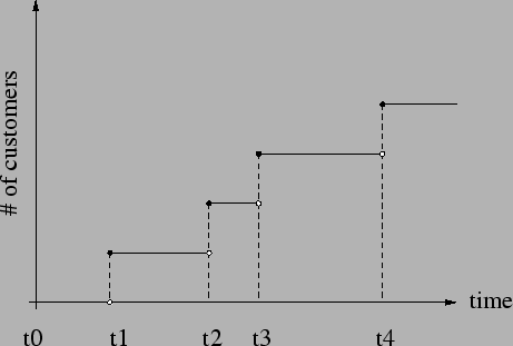 |
Let Fig. 1 be a graph of the customers who are entering a bank.
Every time a customer comes, the counter is increased by one. The time of the
arrival of
 th customer is
  . Since the customers are coming at
random, the sequence
. Since the customers are coming at
random, the sequence
 , denoted shortly
by
, denoted shortly
by
 , is a random sequence. Also, the number of customers
who came in the interval
, is a random sequence. Also, the number of customers
who came in the interval ![$ (t_0, t]$](img6.png) is a random variable
(process). Such a process is right continuous, as indicated by the graph in
Fig. 1.
is a random variable
(process). Such a process is right continuous, as indicated by the graph in
Fig. 1.
As it is often case in the theory of stochastic processes, we assume that
the index set, i.e. the set where
is taking values
from, is
 . Therefore, we have a sequence of non-negative random
variables
. Therefore, we have a sequence of non-negative random
variables
as

WLOG1 let  and
and
 , then
is called a point process (counting process), and is denoted shortly by
, then
is called a point process (counting process), and is denoted shortly by
 .
.
Let
 be inter-arrival time, then the sequence of
inter-arrival times
be inter-arrival time, then the sequence of
inter-arrival times
 is another stochastic process.
Special case is when
is a sequence of
i.i.d.2 random
variables, then the
sequence  is called a renewal process.
is the associated renewal point process, sometimes also
called renewal process. Also, keep in mind that
is called a renewal process.
is the associated renewal point process, sometimes also
called renewal process. Also, keep in mind that
 .
.
Definition (Poisson process) A point process
is
called a Poisson process if and  satisfies the following
conditions
satisfies the following
conditions
- its increments are stationary and its non-overlapping increments are
independent
-
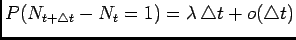
-
Remarks
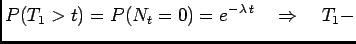
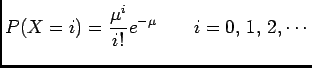
Theorem Let
be a Poisson process, then
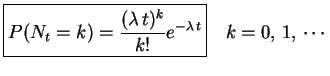 |
(1) |
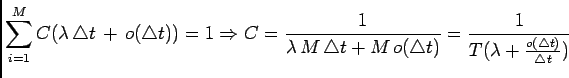
The expression on the left hand side of (1) represents the
probability of  arrivals in the interval
 ![$ (0, t]$](img34.png) .
.
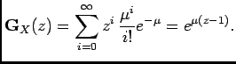
Proof A generating function of a discrete random variable  is
defined
via the following z-transform (recall that the moment generating function of a
continuous random variable is defined through Laplace transform):
is
defined
via the following z-transform (recall that the moment generating function of a
continuous random variable is defined through Laplace transform):
where
 . Let us assume that is a Poisson random variable with
parameter
. Let us assume that is a Poisson random variable with
parameter  , then
and
, then
and
 |
(2) |
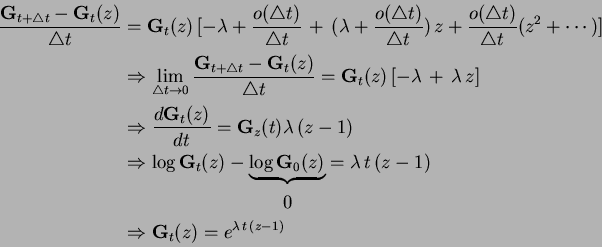
Going back to Poisson process, define the generating function as
Then we can write
Furthermore
Comparing this result to (2) we conclude that  is a Poisson
random variable with parameter
is a Poisson
random variable with parameter
 .
.

Theorem If
is a Poisson process and
 is the inter-arrival time between the
 th and
 th events, then
is a sequence of i.i.d. random variables with exponential
distribution, with parameter
th events, then
is a sequence of i.i.d. random variables with exponential
distribution, with parameter  .
.
Proof
exponential

Figure 2:
Event description
 |
Need to show that  and
and  are independent and is also
exponential.
are independent and is also
exponential.
![$\displaystyle P(T_2>t \vert T_1\in(s-\delta, s+\delta])= \frac{P(T_2>t, T_1\in(s-\delta, s+\delta])}{P(T_1\in(s-\delta, s+\delta])}$](img54.png) |
(3) |
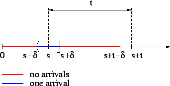
The event
![$ \{T_2>t, T_1\in(s-\delta, s+\delta]\}$](img55.png) is a subset of the event
described by Fig. 2, i.e.
no arrivals one arrival no arrivals
is a subset of the event
described by Fig. 2, i.e.
no arrivals one arrival no arrivals
From (3)

![$\displaystyle P(T_2>t \vert T_1\in(s-\delta, s+\delta]) \le e^{-\lambda (t-2 \delta)}$](img59.png) |
(4) |
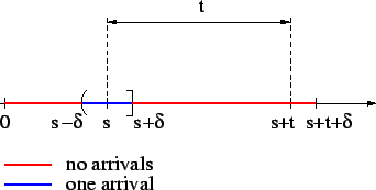
Similarly, the event described by Fig. 3 is a subset of
the event
, therefore
From (3)
![$\displaystyle P(T_2>t \vert T_1\in(s-\delta, s+\delta]) \ge e^{-\lambda t}$](img61.png) |
(5) |
Figure 3:
Event description
 |
From (4) and (5), using squeeze theorem
 , it follows
Therefore, is independent of , and is exponentially
distributed random variable.
, it follows
Therefore, is independent of , and is exponentially
distributed random variable.
Theorem
-
![$ E[N_t]=\lambda t$](img65.png)
-
![$ Var[N_t]=\lambda t$](img66.png)
Proof
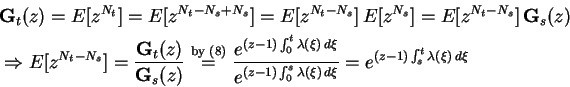
Recall that
![$ \mathbf{G}_t(z)=E[z^{N_t}]$](img67.png) , then
, then
Likewise
Theorem (Conditioning on the number of arrivals) Given that in the
interval ![$ (0, T]$](img70.png) the number of arrivals is
the number of arrivals is  , the
, the  arrival times
are independent and uniformly distributed on
arrival times
are independent and uniformly distributed on ![$ [0, T]$](img73.png) .
.
Proof
Figure 4:
Uniform bins
 |
Independence of arrival times  ,
,  etc. directly follows from
independence of non-overlapping increments. In particular let and
be arrival times of first and second event, then
etc. directly follows from
independence of non-overlapping increments. In particular let and
be arrival times of first and second event, then
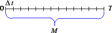
Suppose that we know exactly one event happened in the interval ,
and suppose the interval is partitioned into  segments of length
 , as shown in Fig. 1. Let
  be the probability of
event happening in the
th bin, then
be the probability of
event happening in the
th bin, then
 . From the
definition of Poisson process it follows that
. From the
definition of Poisson process it follows that
 , say
, say
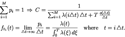
 . The
constant
. The
constant  is determined from
Let be a random variable corresponding to the time of arrival, then
the probability density function (pdf) of can be defined as
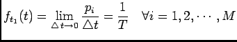 where where |
|
Therefore, is uniformly distributed on .
Let and be the arrival times of two events, and we know exactly two
events happened on . Also assume that and represent mere
labels of events, not necessarily their order. Given that happened in
 th bin, the
probability of occurring in any bin of size
is proportional
to the size of that bin, i.e.
, except for
the
th bin, where
th bin, the
probability of occurring in any bin of size
is proportional
to the size of that bin, i.e.
, except for
the
th bin, where
 . By rendering the bin
size infinitesimal, we notice that the probability remains constant over
all but one bin, the bin in which occurred, where
. By rendering the bin
size infinitesimal, we notice that the probability remains constant over
all but one bin, the bin in which occurred, where  . But this set
is a set of measure zero, so the cumulative sum over again gives
rise to uniform distribution on .
. But this set
is a set of measure zero, so the cumulative sum over again gives
rise to uniform distribution on .
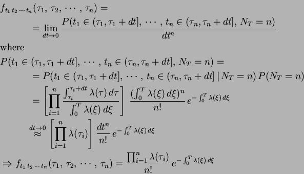
Question
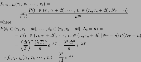
What is the probability of observing events at instances


 on the interval ?
Since arrival times
 are continuous random variables,
the answer is 0. However, we can calculate the associated pdf as
are continuous random variables,
the answer is 0. However, we can calculate the associated pdf as
Question What is the power spectrum of Poisson process?
It does not make sense to talk about the power spectrum of Poisson process,
since it is not a stationary process.
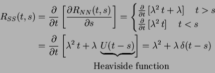
In particular the mean of Poisson process is
and its autocorrelation
function is
Since
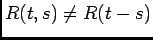 , we conclude that
is
not stationary (in weak sense), therefore it does not make sense to talk about
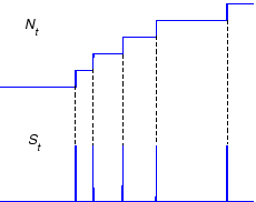
its power spectrum. Let us define the following stochastic process
(Fig. 5)
, we conclude that
is
not stationary (in weak sense), therefore it does not make sense to talk about
its power spectrum. Let us define the following stochastic process
(Fig. 5)
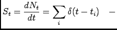 spike train spike train |
(6) |
Figure 5:
Spike train
 |
The fundamental lemma says that if
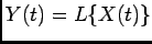 , where
  is a linear
operator, then
is a linear
operator, then
Since differentiation is a linear operator we have
Also, it can be shown using theory of linear operators that
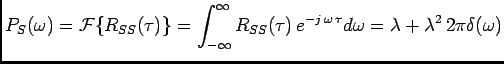
Thus,  is WWS3
stochastic process, and it makes sense to define the power spectrum of such a
process as a Fourier transform of its autocorrelation function i.e.
is WWS3
stochastic process, and it makes sense to define the power spectrum of such a
process as a Fourier transform of its autocorrelation function i.e.
Therefore, the spike train
 of independent times
behaves almost as a white noise, since its power spectrum is flat
for all frequencies, except for the spike at
of independent times
behaves almost as a white noise, since its power spectrum is flat
for all frequencies, except for the spike at  . The process
defined by (6) is
a simple version of what is in engineering literature known as a
shot noise.
. The process
defined by (6) is
a simple version of what is in engineering literature known as a
shot noise.
Definition (Inhomogeneous Poisson process) A Poisson process with a
non-constant rate
 is called inhomogeneous Poisson process.
In this case we have
is called inhomogeneous Poisson process.
In this case we have
- non-overlapping increments are independent (the stationarity is lost though).
-
-
Theorem If
 is a Poisson process with the rate
 , then is a Poisson random variable with parameter
 i.e.
i.e.
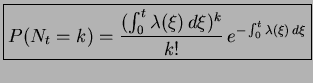 |
(7) |
Proof The proof of this theorem is identical to that of
homogeneous case except that
is replaced by
. In particular,
one can easily get
 |
(8) |
from which (7) readily follows.
Theorem Let
be an inhomogeneous Poisson process with the
rate
and let  , then
 |
(9) |
The application of this theorem stems from the fact that we cannot use
 , since the increments are no longer stationary.
Proof
Thus,  is a Poisson random variable with parameter
 , and (9) easily follows.
Theorem
-
![$ E[N_t]=\int_0^t \lambda(\xi) d\xi$](img126.png)
-
![$ Var [N_t]=\int_0^t \lambda(\xi) d\xi$](img127.png)
Proof Recall that
![$\displaystyle E[N_t]=\left[\frac{dG_z(t)}{dz}\right]_{z=1}$](img128.png) and and![$\displaystyle \quad E[N_t^2]=\left[\frac{d^2G_z(t)}{dz^2}\right]_{z=1}+E[N_t]$](img129.png) |
|
From (8) we have
 , and the two results
follow after immediate calculations.
, and the two results
follow after immediate calculations.
Theorem (Conditioning on the number of arrivals) Given that in the
interval the number of arrivals is , the arrival times
are independently distributed on with the pdf
 .
.
Proof The proof of this theorem is analogous to that of the homogeneous
case. The probability of a single event happening at any of bins (Fig.
1) is given by
 , where
  is the bin index. Given that exactly one event
occurred in the interval , we have
is the bin index. Given that exactly one event
occurred in the interval , we have
The argument for independence of two or more arrival times is identical to that
of the homogeneous case.
Question
What is the probability of observing events at instances
on the interval ?
Since arrival times
are continuous random variables,
the answer is 0. However, we can calculate the associated pdf as
Question How to generate a sample path of a point (Poisson)
process on ? It can be done in many different ways. For a homogeneous
process we use three methods:
- Conditioning on the number of arrivals. Draw the number of arrivals
from a Poisson distribution with parameter
 , and then
draw numbers uniformly distributed on .
, and then
draw numbers uniformly distributed on .
- Method of infinitesimal increments. Partition the segment into
sufficiently small subsegments of length
(say
 ). For each subsegment draw a number
  from a uniform distribution on
 ![$ [0,\,1]$](img139.png) . If
. If
 , an event occurres in
that subsegment. We repeat the procedure for all subsegments. We can use the
approximation
, an event occurres in
that subsegment. We repeat the procedure for all subsegments. We can use the
approximation
 for a less expensive procedure.
- Method of interarrival times. Using the fact that inter-arrival times are
independent and exponentially distributed, we draw random variables
 from exponential distribution with parameter , where
is the smallest integer that satisfies the criterion
from exponential distribution with parameter , where
is the smallest integer that satisfies the criterion
 .
Then the sequence
.
Then the sequence
 generates the required point process.
For an inhomogeneous process, the procedures 1 and 2 can be modified using
the appropriate theory of inhomegeneous Poisson process.
The illustration of the three procedures for a homogeneous case is given below.
We use  and
and
 . For each different procedure
we generate
. For each different procedure
we generate  sample paths, and calculate the statistics by averaging over
ensemble. Raster plots of
sample paths, and calculate the statistics by averaging over
ensemble. Raster plots of  out of samples for the three methods
are shown in Fig. 6, Fig. 7 and Fig. 8,
respectively. Since the generated processes are homogeneous, the inter-arrival
time distribution is exponential with parameter . The histograms
of inter-arrival times corresponding to the three methods are also given below.
They clearly exhibit an exponenital trend. The sample mean and sample standard
deviation (unbiased) are also shown. Keep in mind that for exponentially
distributed random variables, both mean and standard deviation are given by
out of samples for the three methods
are shown in Fig. 6, Fig. 7 and Fig. 8,
respectively. Since the generated processes are homogeneous, the inter-arrival
time distribution is exponential with parameter . The histograms
of inter-arrival times corresponding to the three methods are also given below.
They clearly exhibit an exponenital trend. The sample mean and sample standard
deviation (unbiased) are also shown. Keep in mind that for exponentially
distributed random variables, both mean and standard deviation are given by
 . Sample statistics indicates that is in the
vicinity of
. Sample statistics indicates that is in the
vicinity of  .
.
Figure 6:
Realization of a point process using conditioning on the number of
arrivals. (Top) Ten different sample paths of the same point process
shown as raster plots. (Bottom) The histogram of inter-arrival times, showing
the exponential trend
![\begin{figure}\centering\epsfig{file=rast_homo_1.eps, width=5in} [0.1in]
\epsfig{file=hist_homo_1.eps, width=5.70in}\end{figure}](Timg151.png) |
Figure 7:
Realization of a point process using method of infinitesimal
increments. (Top) Ten different sample paths of the same point process
shown as raster plots. (Bottom) The histogram of inter-arrival times, showing
the exponential trend
![\begin{figure}\centering\epsfig{file=rast_homo_2.eps, width=5in} [0.1in]
\epsfig{file=hist_homo_2.eps, width=5.70in}\end{figure}](Timg152.png) |
Figure 8:
Realization of a point process using method of independent
inter-arrival times. (Top) Ten different sample paths of the same point
process
shown as raster plots. (Bottom) The histogram of inter-arrival times, showing
the exponential trend
![\begin{figure}\centering\epsfig{file=rast_homo_3.eps, width=5in} [0.1in]
\epsfig{file=hist_homo_3.eps, width=5.7in}\end{figure}](Timg153.png) |
Next: About this document ...
Up: Poisson Process, Spike Train
Previous: Poisson Process, Spike Train
Zoran Nenadic
2002-12-13
![$\displaystyle \mathbf{G}_X(z)=E[z^X]=\sum_{i=0}^{\infty}z^i p_i,
$](img36.png)

![\begin{displaymath}\begin{split}P(T_2>t,\,T_1\in(s-\delta,\,s+\delta]) &\le P(T_...
...(s-\delta,\,s+\delta])\,e^{-\lambda\,(t-2\,\delta)} \end{split}\end{displaymath}](img57.png)
![\begin{displaymath}\begin{split}P(N_{s-\delta}=0, \,N_{s+\delta}-N_{s-\delta}=1,...
...mbda\,t}&\le P(T_2>t,\,T_1\in(s-\delta,\,s+\delta]) \end{split}\end{displaymath}](img60.png)
![\begin{displaymath}\begin{split}&\left[\frac{d\mathbf{G}_t(z)}{dz}\right]_{z=1} ...
...a\,t\, e^{\lambda\,t(z-1)}\right]_{z=1}= \lambda\,t \end{split}\end{displaymath}](img68.png)
![\begin{displaymath}\begin{split}&\left[\frac{d^2\mathbf{G}_t(z)}{dz^2}\right]_{z...
...mbda\,t-(\lambda\,t)^2=\lambda\,t \quad\blacksquare \end{split}\end{displaymath}](img69.png)
![\begin{displaymath}\begin{split}&P(t_1\in(0,\,s],\,t_2\in(s,\,t])=P(N_s=1,\,N_t-...
..._s=1\vert N_s=1)=P(t_1\in(0,\,s])\,P(t_2\in(s,\,t]) \end{split}\end{displaymath}](img77.png)
![\begin{displaymath}\begin{split}R(t,s)&\triangleq E[N_t\,N_s]\\ R(t,s)&\overset{...
...lambda^2\,t^2+\lambda\,t=\lambda^2\,t\,s+\lambda\,t \end{split}\end{displaymath}](img98.png)
![$\displaystyle E[S_t]=\frac{d(\lambda t)}{dt}=\lambda$](img105.png)
![\begin{figure}\centering\epsfig{file=rast_homo_1.eps, width=5in} [0.1in]
\epsfig{file=hist_homo_1.eps, width=5.70in}\end{figure}](img151.png)
![\begin{figure}\centering\epsfig{file=rast_homo_2.eps, width=5in} [0.1in]
\epsfig{file=hist_homo_2.eps, width=5.70in}\end{figure}](img152.png)
![\begin{figure}\centering\epsfig{file=rast_homo_3.eps, width=5in} [0.1in]
\epsfig{file=hist_homo_3.eps, width=5.7in}\end{figure}](img153.png)